The Traffic Accident Reconstruction Origin -Article-

The Least Squares Method Applied to Accident Reconstruction

By Bruno Schmidt, PhD

Frequently, when we perform experiments, we can change one of the variables (often called the independent variable) in the experiment, and measure the resulting change (if any) of one of the other variables (called the dependent variable) . For instance, we may:

• change the impact speed of a vehicle with a rigid barrier and record the effect on the resulting crush

  or

• vary the force applied to a bumper isolator and measure the corresponding amount of compression.

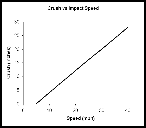
Note that this is not the usual way of displaying crush and speed. The Campbell model typically shows speed on the y-axis and crush on the x-axis. The usual convention is to display the independent variable on the x-axis and the dependent variable on the y-axis. Since for this example, we are talking about changing the impact speed to observe its effect upon crush, the graph does follow the usual convention. In the Campbell discussion of crush, however, he assumes that we have a vehicle whose crush we first measure (in effect, an independent variable) and from which, knowing the crush coefficients, we determine the corresponding barrier speed (the independent variable).

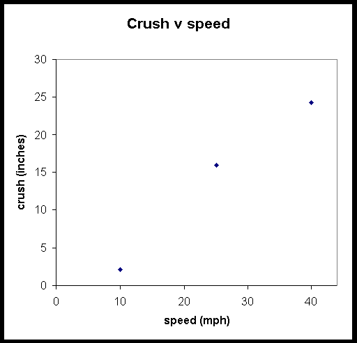
Now, if we make measurements of resulting crush from several different controlled speeds, the variations in measurements and results that are inherent in any real-world experiment will produce a "scatter" of results about the theoretical straight line. For example, assume that we have the following results from a series of three rigid barrier crash tests:

If we plot these values on a graph, we obtain the following result:

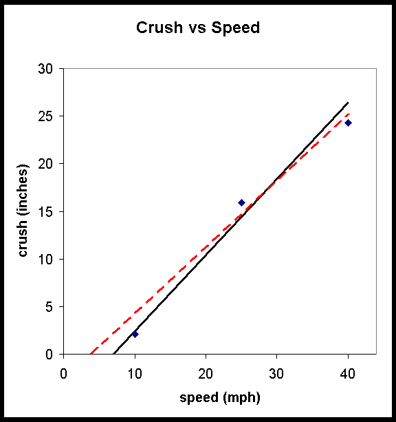
Upon examination of the data points on the graph, we find that they do not follow a perfect line-yet the Campbell model predicts they should. If we try to find the best theoretical fit to the experimental data points, we must ask ourselves, what is the "best" straight line to draw? Two possibilities are shown in the following graph, one for a threshold for crush energy at 7 mph (the solid black line), and one at 4 mph (the dashed red line). The solid black line has a steeper slope-that is, once the threshold is reached, a change in one mph for the impact speed causes more crush than for the dashed red line:

Constructing a Line

• y = mx + b,

where

m is the slope (rise over run) of the line and

b is called the intercept (the value of y when x is zero).

Fitting a Line to Experimental Data

If we do the same set of calculations for the second line, we have this result:

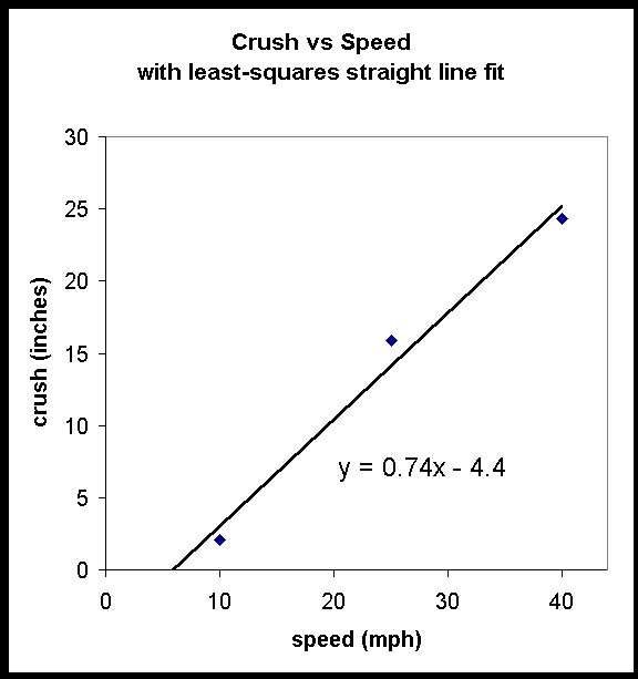
This means that the dashed red line (with m = 0.70 inches/mph and b = -2.8 inches) is a "better fit" to the data than the solid black line (6.66 is less than 7.63). The technique that can be used to find the best fit is to start with a value of m and b and then systematically vary one of those two values until the sum of the squares is a minimum, then systematically vary the other parameter until the sum of the squares is a better minimum, then return to the first parameter and vary it to further improve the minimum, and continue back and forth until no better minimum can be obtained. Fortunately, modern spreadsheets will do that automatically for us. The result of this, with the corresponding equation for the best straight line, is shown in the following graph:

In Microsoft Excel, this is obtained in the Chart menu, where you select Add Trendline. One of the possibilities is a straight line trendline, although a variety of other shapes of lines are possible in Excel. In all cases, however, a least squares fit is used.

Notice that none of the data points lie exactly on the line. Nonetheless, this line still comes closest to all the data points. This is the nature of a least squares fit.

The least squares result for the final spreadsheet trendline is displayed below:

The best previous Error Squared value obtained was 6.66. Clearly the Error Squared of 4.86 calculated using the Excel trendline is smaller and represents a better fit. From this we decide the line determined by a value of m = .74 and b = -4.4 is the best fit for the data.

Finally, we put the m and b values back into the context of our experiment and see that our barrier collision experiments have produced the model:

• Average Crush (inches) = 0.74(inches/MPH) x Speed (MPH) - 4.4 (inches).

which means that entering the value of V in mph into the equation gives the theoretical crush in inches.

Note that this equation can be solved algebraically for the situation where the crush is just zero:

• 0 = 0.74 V - 4.4

• 4.4 = 0.74 V

• 4.4/0.74 = V

• V = 5.9 mph.

Conclusion

Many natural phenomena follow a linear relationship between variables. Hopefully, this discussion of least squares techniques will be helpful to reconstructionists, who wish to relate theoretical formulas to experimental data, in using a systematic, quantitative approach in fitting data to calculations.

Dr. Bruno Schmidt received his Bachelor's degree in mathematics and physics from Cornell College in 1964. His Doctorate degree in physics followed from Iowa State University in 1969. He was a Physics faculty member at Southwest Missouri State University (1969-1984) and head of the Computer Science Department at Southwest Missouri State University (1984-1992). Currently he is Vice President for Academic Affairs at Southwest Missouri State University.

Dr Schmidt has been practicing in the field of accident reconstruction since 1989. He also teaches the Applied Physics for Accident Reconstruction for Texas A&M Engineering Extension Service. He maintains active memberships in S.A.E, Texas Association of Accident Reconstruction Specialists (TAARS) and National Association of Professional Accident Reconstruction Specialists (NAPARS).

He can be reached at [email protected]

Copyright ©