The Traffic Accident Reconstruction Origin -Article-


The Traffic Accident Reconstruction Origin -Article-
|

|
by
Dr. Oren Masory and Bill Wright
Introduction
It is common practice for accident reconstructionists to rely on equations to guide them to some numerical answer. Each of the measured or estimated values that drive the equation will carry some degree of uncertainty. If we are measuring drag factor we may be confident of a value to within +-. 05. If we measure a distance we may be accurate to within +-1 inch. Regardless of how carefully we measure, or how accurate the measuring device, there will always be some level of uncertainty. A change in the value of any of the measured quantities will have some effect on the calculated value. This difference is the "sensitivity" of the equation to the uncertainty. The propagation of this uncertainty to the calculated result should always be considered when expressing the calculated answer. This discussion will center on several methods to quantify this sensitivity to uncertainty.
Sensitivity, An Example Problem
Suppose we are given the task to measure a vehicle's acceleration rate from 0 to 88 ft/sec (60 m/h or 95 km/h). After some thought the following test set up is chosen. A flat vacant roadway is located. The driver points the car down the roadway with a stopwatch in one hand. When ready he floorboards the accelerator and starts the stopwatch in the same instant. The driver watches the speedometer climb 40, 50, 55, 58, 59,60. Just as the needle passes 60 m/h he clicks the stopwatch a second time. He now has the time necessary to accelerate to a known velocity, say in this case 8 seconds. This is sufficient information to calculate the average acceleration rate. We use the relationship:
| (1) |  |
Substituting the measured values of 88 ft/sec and 8 seconds into equation 1:
| (2) | 
|
We calculate an answer of 11 ft/sec2 and return to report this acceleration rate. We were grilled about our test method. The question asked is, what if you made a mistake in reading the speedometer? Stated another way we have been asked to assess how sensitive this equation is to uncertainty in velocity. The difference in speed may make a large difference in acceleration or a small difference. Just looking at the numbers there is no way to know. To answer this question we choose to calculate several different values of acceleration using several different speeds.
First we must choose a range to "bracket". We choose to calculate the change in acceleration for increments 4 ft/sec around our time of 88 ft/second. 4 ft/sec is roughly equivalent to 2 M/h or 4km/h. This increment was chosen because it is a fair estimate for the uncertainty in reading the speedometer. Given this increment, we will calculate a table of acceleration values by holding the measured 8 seconds as constant, and varying values of velocity by values of 4 ft/sec.
That table Follows.
| Velocity ft/sec | Time sec | acceleration ft/sec2 |
| 56 | 8 | 7.00 |
| 60 | 8 | 7.50 |
| 64 | 8 | 8.00 |
| 68 | 8 | 8.50 |
| 72 | 8 | 9.00 |
| 76 | 8 | 9.50 |
| 80 | 8 | 10.00 |
| 84 | 8 | 10.50 |
| 88 | 8 | 11.00 |
| 92 | 8 | 11.50 |
| 96 | 8 | 12.00 |
| 100 | 8 | 12.50 |
| 104 | 8 | 13.00 |
| 108 | 8 | 13.50 |
| 112 | 8 | 14.00 |
| 116 | 8 | 14.50 |
| 120 | 8 | 15.00 |
Table 1
The table tells us that for every change of 4 ft/sec the acceleration changes by .5 ft/sec2. Dividing by 4 will give the change in acceleration for every 1ft/sec. This result is .125 ft/sec2. It appears that a small error in velocity will result in a small error in the resulting calculation for acceleration. This is encouraging. The table has been helpful. But we could use the data in the table differently. We could plot the points and view them graphically.

Fig 1
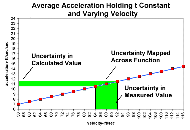
Fig 1 shows the table data plotted. Here acceleration is plotted as a function of velocity. This graph is a "picture" of the relationship expressed in eq. 1 where acceleration is a function of velocity. We can see that it plots as a line. The range of 88 ft/sec +- 4 ft/sec has been highlighted. This is the proposed range of uncertainty. The lines that form this range are velocity values projected vertically up onto the function (the blue line), then mapped perpendicularly onto the acceleration axis. We can see that 84 ft/sec maps to 10.5 ft/sec2 and 92 ft/sec maps to 11.5 ft.sec2
Looking more closely at Fig 1 we see the function that is sloped upward and to the right. When talking about graphs, the word slope has a very specific meaning. It is defined as rise/run, or the change in the y value divided by the change in the x value (where y=f(x)). Slope is usually assigned the variable m. We can use the data from the table to calculate the slope of this function.
For example we choose to find the slope using the two points when V = 84 where a = 10.5 and when V= 88 and a = 11
(3) m = change in y / change in x
Substituting and solving we find
| (4) | 
|
The units of slope in this problem are worth examining. Slope is always rise/run. In this case those units are acceleration/velocity, or (ft/sec2) / (ft/sec). This fraction could simplify but it is meaningful in its current form. What this says is that there is a .125 ft/sec2 change in acceleration for every change in velocity of 1 ft/sec. Notice this is exactly what we determined from looking at the table.
The topic of slope is worth a few more words. Negative slopes indicate lines that decrease in y values as x values increase (go down and to the right). The larger the absolute value of the slope (big positive numbers or small negative numbers) the more steeply the line is angled to the horizontal. Conversely, the smaller the slope (closer its value is to 0) the more horizontal the line. Notice also, since this function is a straight line (has constant slope) we could have calculated the value of m =.125 for the function's slope by using any two points from the table.
We can use the definition of slope in another way. From (3) above slope is defined as
(3) m = change in y / change in x
We can rearrange and write
(5) m (change in x) = change in y
Now recognize that change in x is the uncertainty in the measured value. Change in y is the propagation of this uncertainty, mapped across the function, to the calculated value. This mapping of values across the function is the uncertainty in the calculated value. We can choose a convenient unit value for the uncertainty in x, in this case 1 ft/sec. Once this is done the amount of uncertainty in y is the result of the functions manipulation of x, or its sensitivity. Equation (5) above says that sensitivity is proportional to slope.

Fig 2a Large Slope, Large Sensitivity |

Fig 2b Moderate Slope, Moderate Sensitivity |
Fig 2c Small Slope, Small Sensitivity |
This relationship can also be seen graphically in Fig 2a, 2b and 2c. These figures show a sketch of three hypothetical functions (red lines) with different slopes. First notice the uncertainty in the measured value (x) is the same in all three figures. It is apparent from the graphs that uncertainty maps across these functions very differently. Functions with large slopes map to large uncertainties in the calculated value. Functions with small slopes map to small uncertainties. This is just the graphic representation of equation (5). Again, sensitivity is proportional to the slope of the function.
Confident that our test method is valid we return to report that the function (a = V/t) is not particularly sensitive to errors in velocity measurement. The question fires back, what if you made an error in the measurement of time? This is a different question than we have just answered. This question asks for the sensitivity of the function to uncertainty in time. Let's follow the same method used for checking the sensitivity to velocity.
As before, first we create a table. This time we calculate acceleration holding velocity constant and varying time. For this table we will check the acceleration value every half-second. That table follows
| Velocity ft/sec | Time sec | acceleration ft/sec2 |
| 88 | 4 | 22.00 |
| 88 | 4.5 | 19.56 |
| 88 | 5 | 17.60 |
| 88 | 5.5 | 16.00 |
| 88 | 6 | 14.67 |
| 88 | 6.5 | 13.54 |
| 88 | 7 | 12.57 |
| 88 | 7.5 | 11.73 |
| 88 | 8 | 11.00 |
| 88 | 8.5 | 10.35 |
| 88 | 9 | 9.78 |
| 88 | 9.5 | 9.26 |
| 88 | 10 | 8.80 |
| 88 | 10.5 | 8.38 |
| 88 | 11 | 8.00 |
| 88 | 11.5 | 7.65 |
| 88 | 12 | 7.33 |
Table 2
Examining the data we see that acceleration changes by 4.4 ft/sec2
(.14g) in the first second (from t = 4 to t = 5). This is a significant error. Something
else is troubling about the data in this table. While the change in acceleration in the
first second is 4.4 ft/sec2 the change in the last second (t = 11 to t = 12) is only .67
ft/sec2 (.02g). The meaning of this difference is clear when the data is plotted.
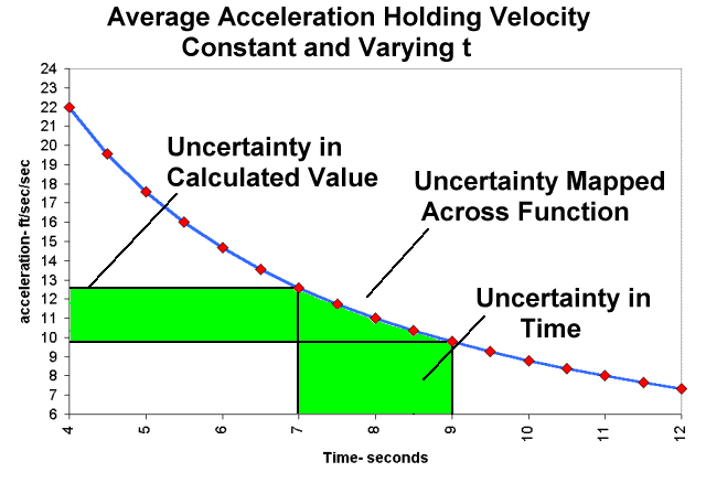
This function plots as a curve rather than a line.

How are we to apply the relationship of sensitivity discussed above to this figure? Stated another way, how do we find the slope of a curve?
The definition of slope is unchanged:
(3) m = change in y / change in x
Using the data from the table, the calculated slope of the first second (t = 4 to t = 5) is
| (6) |
|
We also need to find the value of slope around our point of interest where time equals 8 seconds. We will use the data for the second that begins a half second before our time of t = 8 seconds and ends at the half second after t = 8 seconds (t = 7.5 to t = 8.5). That slope is
| (7) |
|
Looking further down the curve we see the last second of data (t = 11 to t = 12) yields a slope of
| (8) |
|
Examining these numbers we see that the magnitudes of the slopes seem to agree with the graph. That is, the absolute value of the slopes become smaller and smaller as we move to the right (the curve is becoming more horizontal). The negative slopes also make sense. Everywhere the acceleration values decrease as the time values increase (the curve always goes down and to the right). But what to do about the changing slope? We could graphically draw the ranges as was done in the previous example. These ranges are included in green in the Figure 3. We can see from both the table and the graph that 8 sec +- 1 second yields a range of accelerations of 9.78 to 12.57 ft/sec2. But that is only the range for our 8-second car. If the car we had tested was quicker, it could be in the mid 4 second range. Conversely, if it was a very slow accelerating car it could be well beyond the hypothetical 11-12 second range included in the table. There must be an easier way to find sensitivity than calculating, tabulating and graphing values.
A Different Approach to Slope
In fact there is an easier way. We have seen in the previous examples that sensitivity is proportional to slope. What is needed is a way to find he slope of a function at a particular point. This is precisely what a derivative does.
Books are written about derivatives and how to find them. It is calculus. The topic is beyond the scope of this treatment. Suffice it to say:
a) If it doesn't move in our time increment of 0 seconds, why aren't all instantaneous speeds equal to 0?
b) If it moves any distance at all in our 0 length time increment how can it have a speed less than infinity (small number/0 = infinity)?
Let's reexamine the problems above using derivatives.
The relationship is
Average acceleration = Change in Velocity / Change in time
The function is:
| (1) |  |
One derivative of this function is
| (9) |
|
We need more information about this notation.
 is read as the first partial
derivative of acceleration with respect to velocity. Remember we can think of it as the
slope of the function (1) at any value of velocity. Note also the units carry with the
arguments. Here the units of
 are ft/sec2 / ft/sec. Again, as we saw above, this
derivative will be in the units we desire, change in acceleration per change in velocity.
Notice also in the derivative that the slope is not a function of velocity. That means the
that slope is constant as seen above. In other words, the fact that we wanted
acceleration from 0 to 88 ft/sec made no difference to the tests
sensitivity to velocity.
The other derivative is
| (10) |
|
Here
 is read as the first partial derivative of acceleration with respect to
time.
Let's take our test setup and use derivatives to determine the function's sensitivity to each variable. First we will examine the test setup's sensitivity to changes in velocity. From above that partial derivative is
| (9) |
|
Next we substitute and solve with the value of t (8 seconds)
| (11) |
|
We see that this is exactly the same answer we found from the table, the graph, and when we calculated the slope in Eq. 4.
Next the sensitivity to time. That partial derivative is
| (10) |
|
Substitute our values for t and V (8 and 88 respectively) to find the slope for the function at our test values
| (12) |
|
The value calculated from the derivative of -1.375 is very close to the slope we calculated from data in the table (Eq 8) where we found the slope to be -1.38. In fact the slope obtained from the derivative (Eq. 12) is more accurate that the slope obtained from the data. This is due to the fact that slope of the curve changes constantly, even in the small increment of time from 7.5 to 8.5 seconds. Notice also, unlike the speed case for acceleration (Eq. 9 where slope (the derivative) is dependent on time alone), the time sensitivity case is dependent on both time and velocity.
Checking the value of the two derivatives we see the magnitude of
 is greater than the magnitude of
 . Stated another way,
 where
where
 is the absolute value of -1.375. Therefore, we know that the function, and our test,
is most sensitive to unit errors of time.
Applying the Derivatives the Problem at Hand
Earlier we had estimated the accuracy of the time and velocity measurements. We said that velocity was 88 ft/sec +- 4 ft/sec. We also said that our time measurement was 8 sec +- 1 sec. Remember the +- values are the uncertainty in the measured values. We can use the value of the derivatives calculated above (Eqs 11 and 12) to calculate the total uncertainty in the test.
Eq 11 tells us that there is .125ft/sec2 for every 1ft/sec of error. Finding the error for 4 ft/sec is just a matter of multiplying the unit value of the derivative (Eq 11) times the uncertainty.
| (13) |
|
Fortunately we have guessed the uncertainty in time at the unit value of 1 sec.
| (14) |
|
Consequently, the value calculated in eq 12 (
 ) will be our acceleration uncertainty.
The total uncertainty in the test is the sum of uncertainty in acceleration due to uncertainty in velocity (.5ft/sec2) plus the uncertainty in acceleration due to uncertainty in time (1.375ft/sec2).
| (15) |
|
Finally, we can now report completely that the acceleration rate of our car was 11 ft/sec2+- 1.875 ft/sec2 (.34g +-.06g).
Conclusion
Much of common Traffic Accident Reconstruction folklore is explained by circumstances where slope is large, and sensitivity is great.
All of these cases have function derivatives with large slope at their cautioned value.
The reader is cautioned that using a derivative to calculate the uncertainty is only half of the error analysis story. Remember, in this example we guessed at the uncertainty in the measured value. Statistics gives us the tools to make these estimated values credible. That is a topic for another discussion.
Statistics aside, the sensitivity of a particular function to uncertainty is always proportional to its slope at the point of interest. The partial derivative of the function offers a quick and convenient way to assess the function's sensitivity to uncertainty.Dr. Oren Masory is a Professor and the Director Robotics Center of the College of Mechanical Engineering Department at Florida Atlantic University in Boca Raton, FL. He can be reached at (561) 297-2693 or via Email at [email protected]
Bill Wright is an accident investigator with the Palm Beach County Sheriffs Office in West Palm Beach, Fl (USA). He teaches accident investigation and driver training topics. He can be reached at [email protected]
|
Copyright ©
|